Math Primer

How to read this

This primer covers the math the framework uses, no more. It is for readers who are smart but rusty — the equations in the Technical Reference assume graduate-level physics fluency, and that's a steep ramp for anyone whose last differential geometry course was a long time ago, or never happened.

Each entry below is a single concept. The pattern is the same throughout: definition, an intuition you can carry around, a small example, then a pointer to the place in the Technical Reference where the concept gets used. Read the ones you need. Skip what you already know.

Rough triage:

• If you have a graduate physics background, you can skim or skip the whole primer.
• If you have undergraduate physics, the entries on projective spaces, fiber bundles, Kähler structure, and Berry phase are probably the ones worth your time.
• If you're coming from outside physics, work through in order. Total reading time is about an hour.

The primer does not derive PPM. It supplies the vocabulary you need to read PPM. The framework's own claims, derivations, and predictions live in the Technical Reference and the computational notebooks.

1. Sets, functions, and equivalence relations

A set is a collection of objects. A function $f \colon A \to B$ assigns each element of $A$ to a single element of $B$. An equivalence relation on a set is a rule that groups elements into "same" classes — formally, a relation $\sim$ that is reflexive ($x \sim x$), symmetric ($x \sim y \Rightarrow y \sim x$), and transitive ($x \sim y$ and $y \sim z \Rightarrow x \sim z$).

Given an equivalence relation on $A$, the quotient set $A / {\sim}$ is the set of equivalence classes — one point for each "same" group.

This idea is the engine of the next two entries. Manifolds use it to glue local patches; projective spaces are entire spaces built by quotienting.

2. Manifolds

A manifold is a space that, near any chosen point, looks like flat $\Rtwo^n$ for some fixed $n$. The dimension $n$ is the same everywhere on the manifold. Globally the space can be curved or twisted; locally it always looks flat.

Standard examples: a circle is a 1-manifold, the surface of a sphere is a 2-manifold, ordinary 3D space is a 3-manifold, spacetime is a 4-manifold.

A smooth manifold has the additional property that the local flat patches glue together compatibly enough to do calculus globally. Most of physics happens on smooth manifolds. The framework's arena $\CPthree$ is a smooth manifold of real dimension 6 — three complex coordinates, each contributing two real dimensions. Its actuality subspace $\RPthree$ is a smooth manifold of real dimension 3.

3. Projective spaces

A projective space identifies points that lie on the same line through the origin.

Real projective space $\RP^n$ is the set of lines through the origin in $\Rtwo^{n+1}$. Equivalently, take the unit sphere $S^n$ and glue antipodal points together. So $\RP^1$ is a circle; $\RP^2$ is a closed surface (the famous one with no boundary that can't sit in 3D space without self-intersecting); $\RPthree$ is a 3-manifold homeomorphic to the rotation group $SO(3)$.

Complex projective space $\CP^n$ is the analogous construction for complex lines: the set of complex lines through the origin in $\Ctwo^{n+1}$. $\CP^n$ has real dimension $2n$, so $\CPthree$ is six-real-dimensional.

Projective spaces appear in physics whenever two states differing only by an overall scale represent the same physical situation. In quantum mechanics, the states $|\psi\rangle$ and $\lambda|\psi\rangle$ describe the same physics for any nonzero $\lambda$ — so the actual state space of a quantum system is a projective Hilbert space.

4. Group actions and quotient spaces

A group is a set $G$ with a multiplication that has an identity element, inverses, and is associative. The simplest nontrivial example is $\Ztwo = \{e, \sigma\}$ with $\sigma^2 = e$: two elements, the identity and one nontrivial element that squares to the identity.

A group action of $G$ on a space $X$ is a way for each group element to move points around in $X$, consistent with the group's multiplication: for each $g \in G$ there's a map $x \mapsto g \cdot x$, and $(gh) \cdot x = g \cdot (h \cdot x)$.

The quotient space $X / G$ identifies points connected by the action: $x \sim g \cdot x$ for every $g$. So $X / G$ is the space of orbits — each point of the quotient corresponds to one full orbit in $X$.

Projective spaces themselves are quotients: $\CP^n = (\Ctwo^{n+1} \setminus \{0\}) / \Ctwo^*$, where $\Ctwo^*$ acts by scaling.

5. Involutions and fixed points

An involution is a map that's its own inverse: $\tau \circ \tau = \mathrm{id}$. Apply it twice and you're back where you started.

The fixed-point set $\mathrm{Fix}(\tau) = \{p : \tau(p) = p\}$ is the subset of points unmoved by $\tau$.

Examples: reflection across a line in the plane is an involution; its fixed-point set is the line itself. Complex conjugation $z \mapsto \bar z$ on $\Ctwo$ is an involution; its fixed-point set is the real line $\Rtwo \subset \Ctwo$.

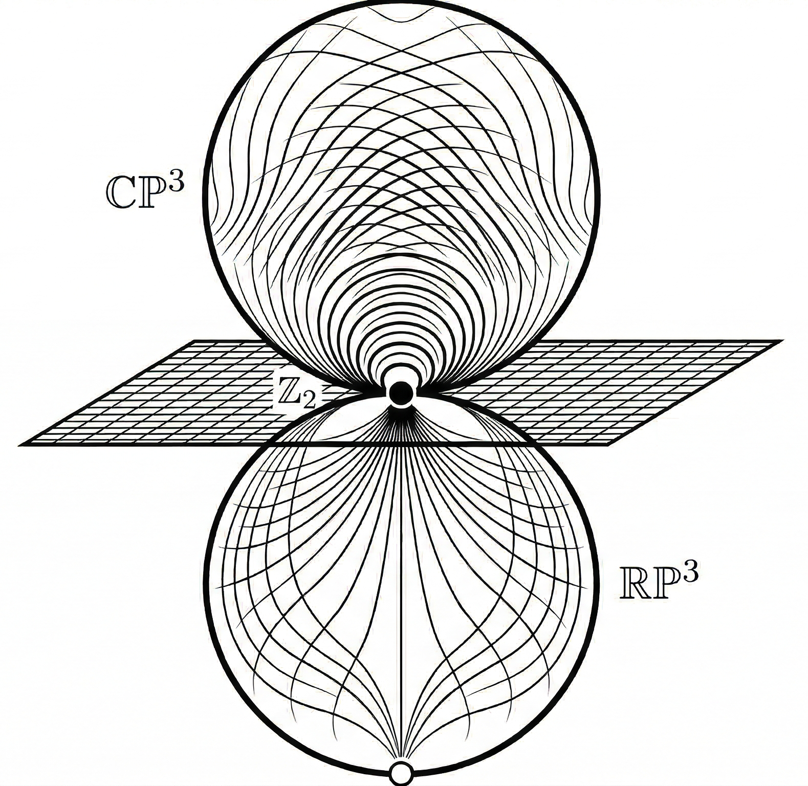
The framework's foundational construction is one specific involution: the anti-holomorphic map $\tau \colon \CPthree \to \CPthree$ that sends each point to its complex conjugate. Its fixed-point set is exactly $\RPthree \subset \CPthree$. So actuality is geometrically a fixed-point set; $\tau$-projection events take a complex possibility-space point and project it onto its real fixed-point shadow.

6. Fiber bundles

A fiber bundle is a space $E$ that, near each point of a base space $B$, looks like a product $B \times F$, where $F$ is the fiber. Globally, the bundle may be twisted — so $E$ is locally but not globally a product.

Trivial example: a cylinder is a fiber bundle with $B$ = circle, $F$ = line segment. Locally, globally, everywhere: just circle × segment.

Non-trivial example: a Möbius strip. Same base (circle), same fiber (segment), but with a global twist that makes it a different bundle. You cannot draw a continuous "top edge" line all the way around without ending up at the bottom.

A section of a bundle is a continuous choice of one point in each fiber — like a curve that hits every fiber exactly once. Some bundles admit many sections; some admit none. The Möbius strip admits sections (you can pick a point on the segment in each fiber). The "hairy ball theorem" says the unit-tangent-vector bundle of $S^2$ admits no continuous nonvanishing section — every haircut on a sphere has a cowlick.

In gauge theory, fields are sections of bundles whose fiber is a Lie group. Electromagnetism is the geometry of $U(1)$ bundles over spacetime; the strong force is $SU(3)$ bundles.

7. Volumes and integration on manifolds

To talk about "the volume of $\RPthree$," you need a notion of integration on a manifold. For a Riemannian manifold (one equipped with a notion of distance), volume comes from a volume form — a way to assign a positive number to each tiny patch consistent with the local metric. Integrating the volume form over a region returns the volume of the region.

$\RPthree$ inherits a natural volume from the unit 3-sphere: $\mathrm{Vol}(\RPthree) = \pi^2$ (half the volume of $S^3$, since $\RPthree = S^3 / \Ztwo$). $\CPthree$ inherits volume from the Fubini–Study metric.

Volumes appear in PPM because dimensionless ratios of geometric volumes set physical constants. The fine-structure constant in particular has expressions involving the ratio $\mathrm{Vol}(\RPthree) / \mathrm{Vol}(\CPthree)$.

8. Topological invariants

Two manifolds are topologically equivalent if one can be deformed continuously into the other without cutting or gluing. Geometric quantities like length, area, and angle generally change under such deformations. The numbers that don't change are topological invariants.

The simplest is connectedness — does the space come in one piece, or several?

The Euler characteristic $\chi$ is a more refined invariant. For a triangulated surface, $\chi = V - E + F$ (vertices minus edges plus faces). $\chi(\text{sphere}) = 2$, $\chi(\text{torus}) = 0$. For complex projective space, $\chi(\CP^n) = n+1$, so $\chi(\CPthree) = 4$. For $\RP^n$ with $n$ odd, $\chi(\RP^n) = 0$.

Betti numbers $b_k$ count "independent $k$-dimensional holes" in a more refined way. Persistent homology tracks how Betti numbers change as a parameter sweeps over a range — a useful tool for distinguishing structures that look similar pointwise but differ globally.

9. Complex and Kähler structure

A complex manifold has charts taking values in $\Ctwo^n$ glued by holomorphic transition functions — meaning calculus on it can be done with complex derivatives. $\CP^n$ is a complex manifold; so is any smooth complex algebraic variety.

A Kähler manifold has three compatible structures: a complex structure (so it's a complex manifold), a Riemannian metric (so distances exist), and a symplectic form (a closed non-degenerate 2-form, the kind of object that runs Hamiltonian dynamics). The compatibility condition is that the three structures are interrelated through a single tensor — not three independent objects pasted together.

$\CP^n$ with the Fubini–Study metric is the canonical Kähler manifold. The framework lives on $\CPthree$ in this Kähler structure.

10. Lie groups and representations

A Lie group is a group that's also a smooth manifold, with the group multiplication smooth. Examples: $U(1)$ (the circle); $SU(2)$ (the 3-sphere with its multiplication); $SO(3)$ (rotations of $\Rtwo^3$, topologically $\RPthree$); the Standard Model gauge group $SU(3) \times SU(2) \times U(1)$.

A representation of a Lie group is a way of realizing its elements as matrices acting on a vector space. The Standard Model groups act on quark and lepton states via specific representations — quarks are in fundamental representations of $SU(3)$ and $SU(2)$; leptons sit in trivial color representations and so on.

The Lie algebra of a Lie group is the tangent space at the identity, equipped with a bracket. It captures the infinitesimal structure of the group and is generally easier to work with than the group itself. A small group element near the identity is $\exp(\epsilon X)$ for $X$ in the Lie algebra and $\epsilon$ small.

11. Berry phase and holonomy

A Berry phase (or geometric phase) is a phase factor a quantum state acquires when its parameters are slowly varied around a closed loop. The state returns to itself in magnitude, but rotated by a phase that depends only on the path, not on how fast it was traversed.

More generally, holonomy is the failure of parallel transport in a fiber bundle to be path-independent. In a curved bundle (one with nontrivial connection), transporting around a loop can leave you rotated relative to where you started. The amount of rotation is the holonomy of that loop.

Berry phases are the common origin of the Aharonov–Bohm effect, geometric quantum computation, the integer quantum Hall effect, and many topological phases of matter. They are also responsible for mixing angles in flavor physics: when a state is parallel-transported along a path in a parameter space that connects different flavor eigenstates, the relative phase it picks up determines the mixing.

12. Density matrices and the Born rule

In quantum mechanics, a pure state is a vector $|\psi\rangle$ in a Hilbert space (with $\langle\psi|\psi\rangle = 1$). A mixed state — a probabilistic mixture of pure states — is described by a density matrix $\rho$: a Hermitian, positive-semidefinite operator with $\mathrm{Tr}(\rho) = 1$. Pure states correspond to rank-1 density matrices $\rho = |\psi\rangle\langle\psi|$.

A projection operator $P$ satisfies $P^2 = P$ and $P^\dagger = P$. The Born rule says: when you measure observable $A$ on state $\rho$, the probability of outcome $a$ is $\mathrm{Tr}(P_a \rho)$, where $P_a$ projects onto the eigenspace of $A$ with eigenvalue $a$. After the measurement, the state collapses to $\rho \mapsto P_a \rho P_a / \mathrm{Tr}(P_a \rho P_a)$.

For systems interacting with an environment, the natural generalization of the Schrödinger equation is the Lindblad equation:

The first term is unitary evolution. The dissipative terms describe how the environment kicks the system. The operators $\hat A_b$ are jump operators labeling which interaction channel fires.

13. Variational principles

A variational principle says: out of all possible motions or configurations, the actual one extremizes some functional. Lagrangian mechanics is variational — classical trajectories minimize the action $\int L\, dt$. Hamilton's equations follow.

In thermodynamics, the free energy $F$ is minimized at equilibrium. In statistical mechanics, the partition function generates everything.

In information geometry and Bayesian inference, the variational free energy $F[\rho, \theta]$ measures how badly a model parameterized by $\theta$ fails to match data, with $\rho$ a posterior distribution. Minimizing $F$ over $\theta$ is approximate Bayesian inference. The "free energy principle" of theoretical neuroscience is a special case of this.

The framework uses the same mathematical object (a free energy) for a different purpose than active inference does. PPM's free energy $\mathcal F = -\log \mathrm{Tr}(\hat A_b \rho \hat A_b^\dagger)$ at each $\tau$-event is the surprisal of branch $b$. Minimizing it picks the most-likely actualization branch. This is the Born rule rewritten as an optimization. The variational principle does not produce consciousness; biology is something that exploits conditions made available by it.

14. Renormalization group and running couplings

In quantum field theory, the values of "constants" depend on the energy scale at which you measure them. The running coupling $g(\mu)$ for a gauge field varies with the renormalization scale $\mu$. The renormalization group (RG) describes how couplings flow with scale.

A coupling can run to zero in the UV (asymptotic freedom — this is what the strong force does, which is why quarks are nearly free at very high energies). Or it can run to a Landau pole (electromagnetism, formally — though the pole is so high it's never reached experimentally). Or it can run to a fixed point.

For PPM, this matters because predictions made at the UV scale need to be RG-evolved down to experimental scales. The geometric prediction $\sin^2\theta_W = 3/8$ holds at the GUT scale; running it down to the $Z$ mass via Standard Model RG gives the experimental value $0.231$. Without the RG, the comparison would look like a 60% discrepancy.

15. Shannon entropy and mutual information

Shannon entropy of a probability distribution $p$ on a finite set is

In bits (log base 2), $H$ is the average number of bits needed to specify an outcome drawn from $p$. A uniform distribution over $2^n$ outcomes has entropy $n$. A distribution concentrated on one outcome has entropy zero — there's nothing to specify.

Mutual information $I(X; Y) = H(X) + H(Y) - H(X, Y)$ measures how much knowing $Y$ tells you about $X$. It's symmetric and non-negative. $I(X; Y) = 0$ iff $X$ and $Y$ are independent.

In PPM, these quantities show up everywhere events are counted: per-event information $I(k) = 3 \log_2 R(k)$ measures the bits an actualization carries; channel-capacity language describes consciousness regimes; the per-event entropy production $\Delta S = 3 k_B \ln(2\pi)$ is set by the topology of the projection.

Reference card

The whole framework on one page. With the vocabulary in hand, this should now read.

Arena $\CPthree$ (complex projective 3-space).

Operator $\tau \colon z \mapsto \bar{z}$ (anti-holomorphic involution). $\mathrm{Fix}(\tau) = \RPthree$ is actuality.

Dynamics Kähler flow on $\CPthree$ between $\tau$-events: $$ H_\alpha = -\frac{\hbar^2}{2 m_\pi}\,\nabla^2_{\CPthree} + m_\pi c^2 \log\!\bigl(1 + |z|^2/\lambda_C^2\bigr). $$ $$ \dot{\rho} = -\tfrac{i}{\hbar}[H_\alpha, \rho] + \sum_b \gamma_b\!\left(\hat{A}_b\rho\hat{A}_b^\dagger - \tfrac{1}{2}\{\hat{A}_b^\dagger \hat{A}_b, \rho\}\right). $$

The world is one geometric process: complex possibility space $\CPthree$ projecting, repeatedly, onto its real fixed-point set $\RPthree$ via the involution $\tau$. Every persistent structure — particles, forces, gravity, the cosmological constant, the geometry of conscious experience — emerges from how that projection runs across an energy hierarchy anchored by $m_\pi$.

Events At gravitational rate $\Gamma_G = G m^3 c/\hbar^2$, $\tau$ fires: $\rho \mapsto \hat{A}_b \rho \hat{A}_b^\dagger / \operatorname{Tr}(\hat{A}_b \rho \hat{A}_b^\dagger)$ (Born rule).

Variational principle $\mathcal{F} = -\log \operatorname{Tr}(\hat{A}_b \rho \hat{A}_b^\dagger)$ minimized at each cycle.

$k$-cascade $E(k) = m_\pi (2\pi)^{(\kref - k)/2}$. Anchors: $k = 1$ (Planck, $\sim 10^{19}$~GeV), $k = \kref$ (pion, $m_\pi$), $k \approx 75$ ($T_{\rm match} = 310$~K), $k \approx 80$ (CMB, $2.7$~K).

Per-event duration $\tau_{\mathrm{event}}(k) = \pi\hbar / (2\, E(k))$ (Margolus–Levitin floor).

Resolvability ratio $R(k) = E(k)/(k_B T)$ at ambient $T$; $T_{\rm match}(k) = E(k)/k_B$. $R = 1$ partitions discrete-quantum / transitional / classical-thermal regimes.

Per-event information $I(k) = 3 \log_2 R(k)$ bits across the three real dimensions of $\RPthree$.

Per-event entropy $\Delta S_{\mathrm{event}} = 3\, k_B \ln(2\pi) \approx 5.5\, k_B$ (scale-independent; set by Hopf fiber circumference $2\pi$).

Boundary capacity $N_\infty = \varphi^{392} \approx 8.4 \times 10^{81}$ (static topological invariant; sets $\Lambda$ and the cosmic IR scale).

Empirical anchor $m_\pi = 140$~MeV (the framework's single dimensionful input).